
Using the lpSolve package in R to optimise an electricity system
[This article was first published on The Manipulative Gerbil: Playing around with Energy Data, and kindly contributed to R-bloggers]. (You can report issue about the content on this page here)
Want to share your content on R-bloggers? click here if you have a blog, or here if you don't.
Want to share your content on R-bloggers? click here if you have a blog, or here if you don't.
Reducing carbon emissions is maybe the world’s most pressing challenge at the moment. One obvious avenue for action is the reduction of carbon emissions from electricity generation, which are a significant contributor to global carbon emissions overall. This is particularly true if trends now in place continue undisturbed, with the world relying on electricity to power their devices, for personal comfort (air conditioners) or even for mobility. What kind of trade-offs are desirable when deciding how much electricity to generate? How does a diversity of possible generation sources impact the best possible choice?
In the following blog post, I’m going to show howlpSolve, a packageavailable through CRAN,can be used to arrive at realistic (enough) scenarios which can inform the de-carbonisation debate. Specifically, I will illustrate an example of using Linear Programming to find the best combination of power stations in a given economy. The data I used is from Cyprus, most of the data for which can be found hereand here, but of course any example could work1.
Linear Optimisation or Linear Programming is a method for finding the best possible (or the least-bad) solution fulfilling a strict criterion (later, multiple criteria). In this example, I will use the lpSolve package which implements the simplex algorithm in determining the best choice given a set of constraints. A good place to read up on the fundamentals behind this is here. In our example, the total costs of operating the entire electricity generation system of Cyprus defines our “objective function” to be minimised while the “constraints” are, in the first instance, the minimum amount of electricity generated to meet demand on Cyprus. The rest of this post will assume only a rudimentary understanding of linear programming–not much else is needed–and will try to focus on how to run the model and arrive at some results.
This is a fairly long blog post but in fact I would try to bring down the word count by making a few things clear in these bullet points:
- The “objective function” is a simple sum of the coefficients of the hourly cost per generator per year. There are thus years × generators elements in this function.
- The constraints exist for each year. Each constraint exists for each year during which the model is run, in this case it is 15 years. The constraints are codified in a matrix which is fed into lpSolve.
- Other than the objective function and the constraints, the elements which I look at are: the “right hand side”, which is a vector that contains the elements defining either the maximum or minimum of a given quantity; and the “direction,” which defines whether or not the constraint is a maximum or a minimum. Note that the “direction” of the objective function is distinct here, it tells us if we want to reduce the objective function (true in our case) or maximise it (for example, if our objective function was a plot of the profits of a firm). If we are looking at the prices of a two items, a and b, during one year, a maximum constraint would look like the following:
First, we define a linear equation which sets the quantity for which we want to find the optimum value–which is either a maximum or minimum. In this example, the optimum is the minimum amount of money needed which can monetize the overall operation of the electricity system/country in question. My model uses a linear expression which sums the hourly operating cost of all the generators in a given system during a 15-year period.
We can then add constraints. For example, I want to set a minimum amount of electricity-hours generated. This is coded in units of MWh (the global household average is about 3.5 MWh annually, but it is more than 3 * that in Canada; 1 MWh = 3.6 billion Joules of energy). Later on, I will add constraints which will place a maximum on the number of hours which a given generator can operate during a year. Finally, I will add a maximum constraint of carbon dioxide emissions from the combination of generators in a given year.
From the data available, and a few other resources easily available online2, I drew up the following table showing the type of generator, its capacity and its hourly running costs.
Name of generator | type | Capacity, MW | Hourly running costs, € |
“Sunny” | Solar photovoltaic | 167.5 | 8.67 |
“Windy” | Wind turbines | 148 | 8.35 |
Vasilikos | steam; fuel oil | 390 | 194.74 |
Dhekelia | steam; fuel oil | 360 | 89.88 |
Combustion generator | Internal Combustion Engine | 100 | 74.90 |
Vasilikos II | Closed Cycle Natural Gas | 440 | 141.60 |
Vasilikos III | Open Cycle Natural Gas | 38 | 31.87 |
There are a few things worth pointing out about the above table. Firstly, the solar and wind generators are grouped into individual “generators” although there are in fact multiple generators. This will have an impact on the final results since the system will decide on which generator to rely on based on price, which has the effect of preferring smaller generators.
Let’s move on with the objective function. I have a system with seven (i = 7) generators, each of which will run for x hours during each of j = 15 years. The values of x are in fact determined by the algortihm deployed; what I provide as arguments/parameters to the function are the hourly operating costs of each generator by year. These can be placed in amatrix representing i generators and j :
Let’s say that these were contained in the matrix with the variable name “bmat”3. The matrix of these values can be read into the R working directory and then turned into a vector:
costcoefficients.matrix <- read_xls("linearprogramming.xls", sheet = "costcoefficients")
# Turn the matrix into a vector; note the use of the transpose.
costcoefficients.vector <- as.vector(t(costcoefficients.matrix))
The vector above now has a coefficient which is the hourly operating cost of each generator. The vector is i * j elements long, with each element representing a generator-year. Note that after every j (= 15) elements, the coefficients move on to the next year. We eventually feed that vector into the linear programming function.
# set the direction of the optimisation to a “minimum”–we want the lowest possible costs
# we feed in the objective function
electricitysystem.results <- lpSolve::lp(dir = "min", costcoefficients.vector)
The results produced by lpSolve are kept in the object electricitysystem.results$solution. It is a vector with the same dimensionality as the objective function, and in our case each element defines the number of hours that a generator-year is operational.
Limiting the problem in this way gives a completely unhelpful answer–0. (In fact, using the R package as above gives an error, although that’s avoiding the more fundamental reason of why there is no viable answer yet.) The reason is that all we have done is to direct the algorithm is to minimise the solution based on our objective function, and obviously the best that can be done is to generate no electricity at all from any generator.
So in the next step, we set a minimum amount of total electricity generated in a given year. This is the equivalent of setting the next constraints which the model has to meet. In the system here, we feed these constraints through the constraint matrix. For example, let’s say that in our first year, each of the generators run at their stated capacity. The minimum total generated electricial energy during that year amounts to 4,274,886 MWh (4.27 TWh), which comes from the electricity generation/consumption data for the benchmark year of 2013. This latter value is input into the “right hand side” of the constraints. Meanwhile, in order to fulfill this demand, each of the generators works at its full capacity for a given number of hours–which is what we determine using the system.
The first row of the constraint matrix, which I have called “example1.constraints,” then looks like this:

Note that each of the generator-years which are inactive in year 1 are 0. Each row of the constraint matrix has i (number of generators) by j (here, number of years) elements; we have rows for each constraint which, for now, will be a constraint defining the minimum electrical energy generated each year. For comparison, this is how row 5 of the constraint matrix looks:

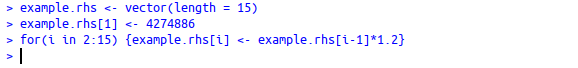
Obviously, the elements where are left as 0 since for a given year, we only care about the relevant generator-years. The first 15 rows of the constraint matrix are constructed in the same way. The next task is to define what the right-hand side of the constraint is–what the minimum value of the electricity generated would be. For the purposes of my model, I allowed the electricity generated to increase by 2% each year. This is coded quite simply as below:
I ought to point out that this is clearly not realistic. If it were, then the demand for electricity generation on Cyprus would grow around nearly ~32% in 15 years, which is really not on the cards in real life, but I wanted to be a bit reckless and illustrate what we get from silly numbers. So this is our Example 1 case: we have electricity demand increasing by 2% each year for 15 years from a base year of 2013. Our objective function remains unchanged from the previous example.
Feeding this in to the console and checking the results is done like this:

There’s one part of the syntax which I did not explain yet, and that’s the “direction” of the constraints, which tells the lpSolve package how to interpret the constraints compared to the right–hand side: are they “>”, “<", ">=” or “<="? For the first case, we have only set a minimum of electricity generated, and so this is going to be defined as:

So, to recap: We have fed in the objective function; the matrix which define the constraints; the “direction,” or the relationship, between what the constraints are, and the constraints on the right-hand side. The results can be accessed from the variable we created above: “example1.results,” and features of it can be accessed using the $ sign: for example, “example1.results$solution” gives an array of the results showing how many hours each of the generators were run, arranged in the same order as the objective function.
Our first set of results are a bit disappointing and, again, meaningless; in fact the only generator to work is the solar farm.

What happened here is that the system simply chooses the most cost effective generator, and also that we did not limit the number of hours in a year, ending with the result that the solar generator runs more than hours than are actually available (8,760) in a year. So our next step is to implement additional constraints which limit the amount which a given generator can run in a particular year.
We can fix this in the system by adding new rows to the constraint matrix; by adding elements to the vector which contains the right hand side values, this time representing the total number of hours which a given generator can run within a set year; and by adding elements to the direction vector, which this time is set as a “maximum” or “>=” instead of the “<=" for the amount of electricity generated.
This time, we will need to add a total of 7 * 15 = 105 rows. Each row will have exactly one element equal to 1, every other element will be 0 since we will define the number of hours for each generator-year separately. For example, the 17th row of additional constraints will contain the constraints for the second year of operation for the second generator, and it looks like this:
Although it looks cumbersome, the additional rows for the constraint matrix can be created in a few short lines of code, like below:
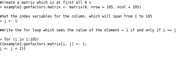
How to define the limits which set out what the maximum number of hours of operation for a given generator in a specific year? For this, I use a pre-defined capacity factor for each generator. In my own example, I actually leave the capacity factor unchanged for each generator over the years, although strictly speaking this is not necessarily accurate. The capacity factor, in this case, is the proportion of hours out of 8760 for which a generator can be turned “on”. In my actual example, I took the values from a spreadsheet which was read into R then multiplied each row–which held the values of the capacity for a given generator–by 8760, giving me a data frame of 105 elements which held the total hours of operation per generator year.
It should be easy enough to see how these are then incorporated into the vector containing the right-hand-side values; for comparison I filled in the total operating hours in the fourth column below. In the case of the solar farm, I allowed the capacity factor to grow by 1.2% per year, while all other capacity factors are held constant for all years of operation.
Generator | Capacity factor (maximum), % | Annual increase (%) | Operating hours/year |
solar | 8.6 | 1.2 | 753-870 |
wind | 14.4 | 1270 | |
Vasilikos I | 75 | stable | 6570 |
Dhekelia | 75 | stable | 6570 |
Internal Combustion Generator | 75 | stable | 6570 |
Vasilikos II | 75 | stable | 6570 |
Vasilikos III | 75 | stable | 6570 |
In other words, I want to allow the thermal (i.e. gas and oil) generators to be running for 75% of the total time of the year. To do this, I set the relevant element in the constraint matrix equal to 1, all other elements in the row are 0. This means that “for generator i in year j, let the total number of hours running equal to CF * 8760 where CF is the maximum capacity factor of that generator. For example, the constraint for the sixth year of the first generator looks like this:

The corresponding entry in the right-hand side vector is then equal to max capacity factor multiplied by 8760 (which for the solar generator in the second year is ~800 hours). This time the chart of operating hours by generator is a little more interesting:
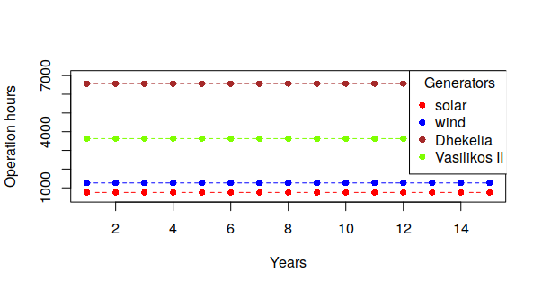
Figure 1: There’s so much wrong in the way this graph is presented that I won’t even mention those things, but the general idea is right here.
What happened here is that the system “chose” different generators to varying extents based not only on how much its hourly operating cost was, but also the extent of time it could reach its capacity. Our third and final run will force the model to take into account an upper limit on the emissions of CO2-equivalent from each generator. I did this by adapting the carbon intensity of each generator—which is the amount of emissions of Greenhouse Gases per unit of energy, expressed in kg/MWh—into a value for each hour running. (This adaptation, again, is important.)
If the limit on carbon emissions for a year j is Mjmegatons, and the emissions from a generator i is given by the coefficient aij, then the emissions cap can be expressed as. The emissions profiles for the generators are in the table below. As before, I add elements to the vector for the right-hand side which contain the caps on the carbon emissions expressed in kgs; the “direction” vector is this time populated with “≤”; and of course there are additional rows to the constraint matrix which contain the coefficients equivalent to the per-hour carbon intensity, the same as in the table below. Note that we can actually change the hourly carbon intensities for different years (but I don’t).
- GeneratorHourly carbon intensity, kg/hour of operationSolar—Wind—Vasilikos I285,870Dhekelia263,880Internal Combustion Generator73,300Vasilikos II158,035Vasilikos III19,497
Obviously I will have to convert the megatons of Cyprus’ carbon emissions from Mtons to kg (1 Mt = 1*109 kg). The value I start with is based on the electricity-generated carbon emissions of Cyprus in 2013 (assuming electric generation was responsible for 50% of Cypriot carbon emissions). I then reduce the caps on successive years by an amount of 2% per step; these values are input into the right-hand side. Remember that here again, the corresponding elements of the direction vector are “<=".
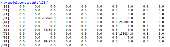
The rows of the constraint matrix which contain the relevant coefficients are again defined by generator-year. This time, all generators contributing to carbon emissions in year j are given the full value (as shown in the table for carbon intensities above) for hourly operation, giving us 15 rows of additional data. For example, the row of data showing carbon intensities in the third year of operation looks like the following:
For this final run, example 3, I am only going to focus on one of the thermal power plants: the natural gas generator at Vasilikos or “Vasilikos I”. The plot below shows how with each successive year, the Vasilikos NG generator acceleratedly approaches its peak capacity of 75%.
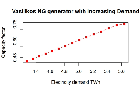
What I wanted to illustrate graphically–because I really should cut down on the use of words right now–is how the load on thermal generators could change when the requirements of a carbon cap are taken into account. Instead of the stable flatline after example 2 above, this time the system utilises generators to differing extents, and it naturally chose the (less carbon intense) natural gas generator over fuel oil generators.
Epilogue and caveats
- There is no way that the above model could be an “accurate” description of the electricity situation in Cyprus, but it is a fun way to start thinking about the choices small island nations need to make when dealing with existing power infrastructures.
- Without a doubt the biggest flaw in the model presented here is that it does not allow for the intermittency of the renewable generators in particular. A more complete/correct system would allow for 8760 hours of each year, then set the caps for the renewable generators based on how much wind and solar power is actually available for a given hour. These data are obtainable from the “Typical Meteorological Year” of Cyprus. The resulting model would of course be much larger in size but not otherwise more complex. I was supposed to start work on such a model, but I’m also about to take my summer holidays, so …
- Another avenue would be to find ways to allow the model to let individual generators only partially on. I think this is a bit more tricky and haven’t fully thought it out yet.
- There are a few consequences of defining the solar farm and wind farm as inidivudal stand-alone generators, but this was done out of expediency and can be easily fixed.
1There are many reasons why Cyprus makes sense. One of them is that the country’s electricity system is considerably outdated, relying almost entirely on fuel oil generators. Another is that, as a small island lacking international infrastructure and power lines, it can serve as a microcosm for isolated locales in many parts of the world.
2It should be easy to find operating prices for a given type of generator. In some cases you have to adapt the running cost per MWh to a running cost per hour.
3In many of the operations of this blog post, matrices and data.frames are more or less interchangeable.
To leave a comment for the author, please follow the link and comment on their blog: The Manipulative Gerbil: Playing around with Energy Data.
R-bloggers.com offers daily e-mail updates about R news and tutorials about learning R and many other topics. Click here if you're looking to post or find an R/data-science job.
Want to share your content on R-bloggers? click here if you have a blog, or here if you don't.