
Time Series Forecasting with XGBoost and Feature Importance
Want to share your content on R-bloggers? click here if you have a blog, or here if you don't.
Those who follow my articles know that trying to predict gold prices has become an obsession for me these days. And I am also wondering which factors affect the prices. For the gold prices per gram in Turkey, are told that two factors determine the results: USA prices per ounce and exchange rate for the dollar and the Turkish lira. Let’s check this perception, but first, we need an algorithm for this.
In recent years, XGBoost is an uptrend machine learning algorithm in time series modeling. XGBoost (Extreme Gradient Boosting) is a supervised learning algorithm based on boosting tree models. This kind of algorithms can explain how relationships between features and target variables which is what we have intended. We will try this method for our time series data but first, explain the mathematical background of the related tree model.
")
- K represents the number of tree
represents the basic tree model.
We need a function that trains the model by measuring how well it fits the training data. This is called the objective function.
 + \displaystyle\sum_{k} \Omega(f_k)")
represents the loss function which is the error between the predicted values and observed values.
is the regularization function to prevent overfitting.
 = \gamma T + \frac{1} {2} \eta||w||^2")
- T represents the leaves, the number of leaf nodes of each tree. Leaf node or terminal node means that has no child nodes.
represents the score (weight) of the leaves of each tree, so it is calculated in euclidean norm.
represents the learning rate which is also called the shrinkage parameter. With shrinking the weights, the model is more robust against the closeness to the observed values. This prevents overfitting. It is between 0 and 1. The lower values mean that the more trees, the better performance, and the longer training time.
represents the splitting threshold. The parameter is used to prevent the growth of a tree so the model is less complex and more robust against overfitting. The leaf node would split if the information gain less than

Now, we can start to examine our case we mention at the beginning of the article. In order to do that, we are downloading the dataset we are going to use, from here.
#Building data frame
library(readxl)

df_xautry <- read_excel("datasource/xautry_reg.xlsx")
df_xautry$date <- as.Date(df_xautry$date)

#Splitting train and test data set
train <- df_xautry[df_xautry$date < "2021-01-01",]
test <- df_xautry[-(1:nrow(train)),]
We will transform the train and test dataset to the DMatrix object to use in the xgboost process. And we will get the target values of the train set in a different variable to use in training the model.
#Transform train and test data to DMatrix form
library(dplyr)
library(xgboost)

train_Dmatrix <- train %>%
                 dplyr::select(xe, xau_usd_ounce) %>%
                 as.matrix() %>%
                 xgb.DMatrix()


pred_Dmatrix <- test %>%
                dplyr::select(xe, xau_usd_ounce) %>%
                as.matrix() %>%
                xgb.DMatrix()

targets <- train$xau_try_gram
We will execute the cross-validation to prevent overfitting, and set the parallel computing parameters enable because the xgboost algorithm needs it. We will adjust all the parameter we’ve just mentioned above with trainControl function in caret package.
We also will make a list of parameters to train the model. Some of them are:
- nrounds: A maximum number of iterations. It was shown by t at the tree model equation. We will set a vector of values. It executes the values separately to find the optimal result. Too large values can lead to overfitting however, too small values can also lead to underfitting.
- max_depth: The maximum number of trees. The greater the value of depth, the more complex and robust the model is but also the more likely it would be overfitting.
- min_child_weight: As we mentioned before with w in the objective function, it determines the minimum sum of weights of leaf nodes to prevent overfitting.
- subsample: It is by subsetting the train data before the boosting tree process, it prevents overfitting. It is executed once at every iteration.
#Cross-validation
library(caret)

xgb_trcontrol <- trainControl(
  method = "cv",
  number = 10,
  allowParallel = TRUE,
  verboseIter = FALSE,
  returnData = FALSE
)

#Building parameters set
xgb_grid <- base::expand.grid(
  list(
    nrounds = seq(100,200),
    max_depth = c(6,15,20),
    colsample_bytree = 1,
    eta = 0.5,
    gamma = 0,
    min_child_weight = 1,
    subsample = 1)
)
Now that all the parameters and needful variables are set, we can build our model.
#Building the model
model_xgb <- caret::train(
  train_Dmatrix,targets,
  trControl = xgb_trcontrol,
  tuneGrid = xgb_grid,
  method = "xgbTree",
  nthread = 10
)
We can also see the best optimal parameters.
model_xgb$bestTune
#  nrounds max_depth eta gamma colsample_bytree min_child_weight #subsample
#1     100         6 0.5     0                1                1         1
To do some visualization in the forecast function, we have to transform the predicted results into the forecast object.
#Making the variables used in forecast object
fitted <- model_xgb %>%
  stats::predict(train_Dmatrix) %>%
  stats::ts(start = c(2013,1),frequency = 12)

ts_xautrygram <- ts(label,start=c(2013,1),frequency=12)
forecast_xgb <- model_xgb %>% stats::predict(pred_Dmatrix)
forecast_ts <- ts(forecast_xgb,start=c(2021,1),frequency=12)

#Preparing forecast object
forecast_xautrygram <- list(
  model = model_xgb$modelInfo,
  method = model_xgb$method,
  mean = forecast_ts,
  x = ts_xautrygram,
  fitted = fitted,
  residuals = as.numeric(ts_xautrygram) - as.numeric(fitted)
)
class(forecast_xautrygram) <- "forecast"
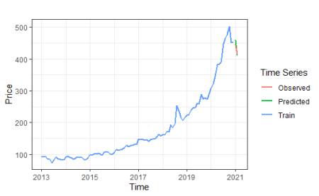
We will show train, unseen, and predicted values for comparison in the same graph.
#The function to convert decimal time label to wanted format
date_transform <- function(x) {format(date_decimal(x), "%Y")}
#Making a time series varibale for observed data
observed_values <- ts(test$xau_try_gram,start=c(2021,1),frequency=12)

#Plot forecasting
library(ggplot2)
library(forecast)

autoplot(forecast_xautrygram)+
  autolayer(forecast_xautrygram$mean,series="Predicted",size=0.75) +
  autolayer(forecast_xautrygram$x,series ="Train",size=0.75 ) +
  autolayer(observed_values,series = "Observed",size=0.75) +
  scale_x_continuous(labels =date_transform,breaks = seq(2013,2021,2) ) +
  guides(colour=guide_legend(title = "Time Series")) +
  ylab("Price") + xlab("Time") +
  ggtitle("") +
  theme_bw()
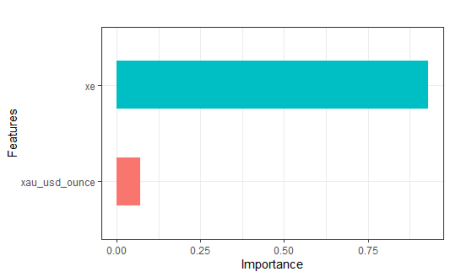
To satisfy that curiosity we mentioned at the very beginning of the article, we will find the ratio that affects the target variable of each explanatory variable separately.
#Feature importance
xgb_imp <- xgb.importance(
  feature_names = colnames(train_Dmatrix),
  model = model_xgb$finalModel)

xgb.ggplot.importance(xgb_imp,n_clusters = c(2))+
  ggtitle("") +
  theme_bw()+
  theme(legend.position="none")

xgb_imp$Importance
#[1] 0.92995147 0.07004853
Conclusion
When we examine the above results and plot, contrary to popular belief, it is seen that the exchange rate has a more dominant effect than the price of ounce gold. In the next article, we will compare this method with the dynamic regression ARIMA model.
References
- Data Side of Life
- Wei Li,Yanbin Yin, Xiongwen Quan and Han Zhang
- Josiah Parry
- XGBoost Documentation
- Analytics Vidhya
R-bloggers.com offers daily e-mail updates about R news and tutorials about learning R and many other topics. Click here if you're looking to post or find an R/data-science job.
Want to share your content on R-bloggers? click here if you have a blog, or here if you don't.