If you want to count the number of days between two dates, you can use the DAYS, DATEDIF, and NETWORKDAYS functions in Google Sheets to do so. DAYS and DATEDIF count all days, while NETWORKDAYS excludes Saturday and Sunday.

Counting All Days Between Two Dates

To count the days between two dates, regardless of whether the day is a weekday or a holiday, you can use the DAYS or DATEDIF functions.

Using the DAYS Function

The DAYS function is the easiest to use, so long as you're not fussed about excluding holidays or weekend days. DAYS will take note of additional days held in a leap year, however.

To use DAYS to count between two days, open your Google Sheets spreadsheet and click on an empty cell. Type

        =DAYS("01/01/2019","01/01/2018")
    

, replacing the dates shown with your own.

Use your dates in reverse order, so put the end date first, and the start date second. Using the start date first will result in DAYS returning a negative value.

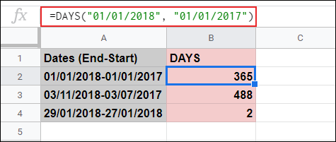
As the example above shows, the DAYS function counts the total number of days between two specific dates. The date format used in the example above is the U.K. format, DD/MM/YYYY. If you're in the U.S., make sure you use MM/DD/YYYY.

You'll need to use the default date format for your locale. If you want to use a different format, click File > Spreadsheet Settings and change the "Locale" value to another location.

You can also use the DAYS function with cell references. If you've specified two dates in separate cells, you can type

        =DAYS(A1, A11)
    

, replacing the A1 and A11 cell references with your own.

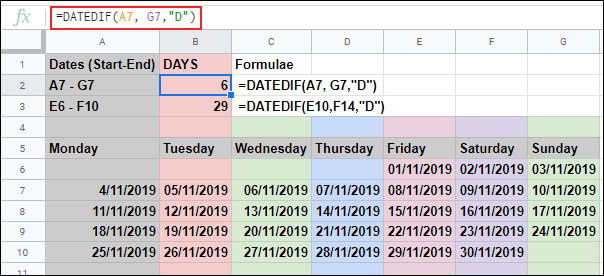
In the example above, a difference of 29 days is recorded from dates held in cells E6 and F10.

Using the DATEDIF Function

An alternative to DAYS is the DATEDIF function, which allows you to calculate the number of days, months, or years between two set dates.

Like DAYS, DATEDIF takes leap days into account and will calculate all days, rather than limit you to business days. Unlike DAYS, DATEDIF doesn't work in reverse order, so use the start date first and the end date second.

If you want to specify the dates in your DATEDIF formula, click on an empty cell and type

        =DATEDIF("01/01/2018","01/01/2019","D")
    

, replacing the dates with your own.

If you want to use dates from cell references in your DATEDIF formula, type

        =DATEDIF(A7,G7,"D")
    

, replacing the A7 and G7 cell references with your own.

Counting Business Days Between Two Dates

The DAYS and DATEDIF functions allow you to find the days between two dates, but they count all days. If you want to count business days only, and you want to discount additional holiday days, you can use the NETWORKDAYS function.

NETWORKDAYS treats Saturday and Sunday as weekend days, discounting these during its calculation. Like DATEDIF, NETWORKDAYS uses the start date first, followed by the end date.

To use NETWORKDAYS, click on an empty cell and type

        =NETWORKDAYS(DATE(2018,01,01),DATE(2019,01,01))
    

. Using a nested DATE function allows you to convert years, months, and dates figures into a serial date number, in that order.

Replace the figures shown with your own year, month, and date figures.

You can also use cell references within your NETWORKDAYS formula, instead of a nested DATE function.

Type

        =NETWORKDAYS(A6,B6)
    

 in an empty cell, replacing the A6 and B6 cell references with your own.

In the above example, the NETWORKDAYS function is used to calculate the working business days between various dates.

If you want to exclude certain days from your calculations, like days of certain holidays, you can add these at the end of your NETWORKDAYS formula.

To do that, click on an empty cell and type

        =NETWORKDAYS(A6,B6,{B6:D6}
    

. In this example, A6 is the start date, B6 is the end date, and the B6:D6 range is a range of cells containing days of holidays to be excluded.

You can replace the cell references with your own dates, using a nested DATE function, if you'd prefer. To do this, type 

        =NETWORKDAYS(E11,F13,{DATE(2019,11,18),DATE(2019,11,19)})
    

, replacing the cell references and DATE criteria with your own figures.

In the above example, the same range of dates is used for three NETWORKDAYS formulae. With 11 standard business days reported in cell B2, between two and three additional holiday days are removed in cells B3 and B4.