The original goal of this post was to explore the relationship between the softmax and sigmoid functions. In truth, this relationship had always seemed just out of reach: "One has an exponent in the numerator! One has a summation! One has a 1 in the denominator!" And of course, the two have different names.
Once derived, I quickly realized how this relationship backed out into a more general modeling framework motivated by the conditional probability axiom itself. As such, this post first explores how the sigmoid is but a special case of the softmax, and the underpinnings of each in Gibbs distributions, factor products and probabilistic graphical models. Next, we go on to show how this framework extends naturally to define canonical model classes such as the softmax regression, conditional random fields, naive Bayes and hidden Markov models.
Our goal
This is a predictive model. It is a diamond that receives an input and produces an output.
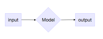
The input is a vector \(\mathbf{x} = [x_0, x_1, x_2, x_3]\). There are 3 possible outputs: \(a, b, c\). The goal of our model is to predict the probability of producing each output conditional on the input, i.e.
Of course, a probability is but a real number that lies on the closed interval \([0, 1]\).
How does the input affect the output?
Our input is a list of 4 numbers; each one affects each possible output to a different extent. We'll call this effect a "weight." 4 inputs times 3 outputs equals 12 distinct weights. They might look like this:
| \(a\) | \(b\) | \(c\) | |
|---|---|---|---|
| \(x_0\) | .1 | .4 | .3 |
| \(x_1\) | .2 | .3 | .4 |
| \(x_2\) | .3 | .2 | .1 |
| \(x_3\) | .4 | .1 | .2 |
Producing an output
Given an input \(x = [x_0, x_1, x_2, x_3]\), our model will use the above weights to produce a number for each output \(a, b, c\). The effect of each input element will be additive. The reason why will be explained later on.
These sums will dictate what output our model produces. The biggest number wins. For example, given
our model will have the best chance of producing a \(c\).
Converting to probabilities
We said before that our goal is to obtain the following:
The \(\mathbf{x}\) is bold so as to represent any input value. Given that we now have a specific input value, namely \(x\), we can state our goal more precisely:
Thus far, we just have \(\{\tilde{a}: 5, \tilde{b}: 7, \tilde{c}: 9\}\). To convert each value to a probability, i.e. an un-special number in \([0, 1]\), we just divide by the sum.
Finally, to be a valid probability distribution, all numbers must sum to 1.
What if our values are negative?
If one of our initial unnormalized probabilities were negative, i.e. \(\{\tilde{a}: -5, \tilde{b}: 7, \tilde{c}: 9\}\), this all breaks down.
\(\frac{-5}{11}\) is not a valid probability as it does not fall in \([0, 1]\).
To ensure that all unnormalized probabilities are positive, we must first pass them through a function that takes as input a real number and produces as output a strictly positive real number. This is simply an exponent; let's choose Euler's number (\(e\)) for now. The rationale for this choice will be explained later on (though do note that any positive exponent would serve our stated purpose).
Our normalized probabilities, i.e. valid probabilities, now look as follows:
More generally,
This is the softmax function.
Relationship to the sigmoid
Whereas the softmax outputs a valid probability distribution over \(n \gt 2\) distinct outputs, the sigmoid does the same for \(n = 2\). As such, the sigmoid is simply a special case of the softmax. By this definition, and assuming our model only produces two possible outputs \(p\) and \(q\), we can write the sigmoid for a given input \(x\) as follows:
Similar so far. However, notice that we only need to compute probabilities for \(p\), as \(P(y = q\vert \mathbf{x}) = 1 - P(y = p\vert \mathbf{x})\). On this note, let's re-expand the expression for \(P(y = p\vert \mathbf{x})\):
Then, dividing both the numerator and denominator by \(e^{\tilde{p}}\):
Finally, we can plug this back into our original complement:
Our equation is underdetermined as there are more unknowns (two) than equations (one). As such, our system will have an infinite number of solutions \((\tilde{p},\tilde{q})\). For this reason, we can simply fix one of these values outright. Let's set \(\tilde{q} = 0\).
This is the sigmoid function. Lastly,
Why is the unnormalized probability a summation?
We all take for granted the semantics of the canonical linear combination \(\sum\limits_{i}w_ix_i\). But why do we sum in the first place?
To answer this question, we'll first restate our goal: to predict the probability of producing each output conditional on the input, i.e. \(P(Y = y\vert \mathbf{x})\). Next, we'll revisit the definition of conditional probability itself:
Personally, I find this a bit difficult to explain. Let's rearrange to obtain something more intuitive.
This reads:
The probability of observing (given values of) \(A\) and \(B\) concurrently, ie. the joint probability of \(A\) and \(B\), is equal to the probability of observing \(A\) times the probability of observing \(B\) given that \(A\) has occurred.
For example, assume that the probability of birthing a girl is \(.55\), and the probability of a girl liking math is \(.88\). Therefore,
Now, let's rewrite our original model output in terms of the definition above.
Remember, we exponentiated each unnormalized probability \(\tilde{y}\) so as to convert it to a strictly positive number. Technically, this number should be called \(\tilde{P}(y, \mathbf{x})\) as it may be \(\gt 1\) and therefore not yet a valid a probability. As such, we need to introduce one more term to our equality chain, given as:
This is the arithmetic equivalent of \(\frac{.2}{1} = \frac{3}{15}\).
In the left term:
- The numerator is a valid joint probability distribution.
- The denominator, "the probability of observing any value of \(\mathbf{x}\)", is 1.
In the right term:
- The numerator is a strictly positive unnormalized probability distribution.
- The denominator is some constant that ensures that
sums to 1. In fact, this "normalizer" is called a partition function; we'll come back to this below.
With this in mind, let's break down the numerator of our softmax equation a bit further.
Lemma: Given that our output function1 performs exponentiation so as to obtain a valid conditional probability distribution over possible model outputs, it follows that our input to this function2 should be a summation of weighted model input elements3.
- The softmax function.
- One of \(\tilde{a}, \tilde{b}, \tilde{c}\).
- Model input elements are \([x_0, x_1, x_2, x_3]\). Weighted model input elements are \(w_0x_0, w_1x_1, w_2x_2, w_3x_3\).
Unfortunately, this only holds if we buy the fact that \(\tilde{P}(a, \mathbf{x}) = \prod\limits_i e^{(w_ix_i)}\) in the first place. Introducing the Gibbs distribution.
Gibbs distribution
A Gibbs distribution gives the unnormalized joint probability distribution over a set of outcomes, analogous to the \(e^{\tilde{a}}, e^{\tilde{b}}, e^{\tilde{c}}\) computed above, as:
where \(\Phi\) defines a set of factors.
Factors
A factor is a function that:
- Takes a list of random variables as input. This list is known as the scope of the factor.
- Returns a value for every unique combination of values that the random variables can take, i.e. for every entry in the cross-product space of its scope.
For example, a factor with scope \(\{\mathbf{A, B}\}\) might look like:
| A | B | \(\phi\) |
|---|---|---|
| \(a^0\) | \(b^0\) | \(20\) |
| \(a^0\) | \(b^1\) | \(25\) |
| \(a^1\) | \(b^0\) | \(15\) |
| \(a^1\) | \(b^1\) | \(4\) |
Probabilistic graphical models
Inferring behavior from complex systems amounts (typically) to computing the joint probability distribution over its possible outcomes. For example, imagine we have a business problem in which:
- The day-of-week (\(\mathbf{A}\)) and the marketing channel (\(\mathbf{B}\)) impact the probability of customer signup (\(\mathbf{C}\)).
- Customer signup impacts our annual recurring revenue (\(\mathbf{D}\)) and end-of-year hiring projections (\(\mathbf{E}\)).
- Our ARR and hiring projections impact how much cake we will order for the holiday party (\(\mathbf{F}\)).
We might draw our system as such:

Our goal is to compute \(P(A, B, C, D, E, F)\). In most cases, we'll only have data on small subsets of our system; for example, a controlled experiment we once ran to investigate the relationships between \(A, B, C\), or a survey asking employees how much cake they like eating at Christmas. It is rare, if wholly unreasonable, to ever have access to the full joint probability distribution for a moderately complex system.
To compute this distribution we break it into pieces. Each piece is a factor which details the behavior of some subset of the system. (As one example, a factor might give the number of times you've observed \((\mathbf{A} > \text{3pm}, \mathbf{B} = \text{Facebook}, \mathbf{C} > \text{50 signups})\) in a given day.) To this effect, we say:
A desired, unnormalized probability distribution \(\tilde{P}\) factorizes over a graph \(G\) if there exists a set of a factors \(\Phi\) such that
$$ \tilde{P} = \tilde{P}_{\Phi} = \prod\limits_{i=1}^{k}\phi_i(\mathbf{D}_i) $$where \(\Phi = \{\phi_1(\mathbf{D_1}), ..., \phi_k(\mathbf{D_k})\}\) and \(G\) is the induced graph for \(\Phi\).
The first half of this lemma does nothing more than restate the definition of an unnormalized Gibbs distribution. Expanding on the second half, we note:
The graph induced by a set of factors is a pretty picture in which we draw a circle around each variable in the factor domain superset and draw lines between those that appear concurrently in a given factor domain.
With two factors \(\phi(\mathbf{A, B}), \phi(\mathbf{B, C})\) the "factor domain superset" is \(\{\mathbf{A, B, C}\}\). The induced graph would have three circles with lines connecting \(\mathbf{A}\) to \(\mathbf{B}\) and \(\mathbf{B}\) to \(\mathbf{C}\).
Finally, it follows that:
- Given a business problem with variables \(\mathbf{A, B, C, D, E, F}\) — we can draw a picture of it.
- We can build factors that describe the behavior of subsets of this problem. Realistically, these will only be small subsets.
- If the graph induced by our factors looks like the one we drew, we can represent our system as a factor product.
Unfortunately, the resulting factor product \(\tilde{P}_{\Phi}\) is still unnormalized just like \(e^{\tilde{a}}, e^{\tilde{b}}, e^{\tilde{c}}\) in our original model.
Partition function
The partition function was the denominator, i.e. "normalizer", in our softmax function. It is used to turn an unnormalized probability distribution into a normalized (i.e. valid) probability distribution. A true Gibbs distribution is given as follows:
where \(\mathbf{Z}_{\Phi}\) is the partition function.
To compute this function, we simply add up all the values in the unnormalized table. Given \(\tilde{P}_{\Phi}(\mathbf{X_1, ..., X_n})\) as:
| A | B | \(\phi\) |
|---|---|---|
| \(a^0\) | \(b^0\) | \(20\) |
| \(a^0\) | \(b^1\) | \(25\) |
| \(a^1\) | \(b^0\) | \(15\) |
| \(a^1\) | \(b^1\) | \(4\) |
Our valid probability distribution then becomes:
| A | B | \(\phi\) |
|---|---|---|
| \(a^0\) | \(b^0\) | \(\frac{20}{64}\) |
| \(a^0\) | \(b^1\) | \(\frac{25}{64}\) |
| \(a^1\) | \(b^0\) | \(\frac{15}{64}\) |
| \(a^1\) | \(b^1\) | \(\frac{4}{64}\) |
This is our denominator in the softmax function.
*I have not given an example of the actual arithmetic of a factor product (of multiple factors). It's trivial. Google.
Softmax regression
Once more, the goal of our model is to predict the probability of producing each output conditional on the given input, i.e.
In machine learning training data we're given the building block of a joint probability distribution, e.g. a ledger of observed co-occurences of inputs and outputs. We surmise that each input element affects each possible output to a different extent, i.e. we multiply it by a weight. Next, we exponentiate each product \(w_ix_i\), i.e. factor, then multiply the results (alternatively, we could exponentiate the linear combination of the factors, i.e. features in machine learning parlance): this gives us an unnormalized joint probability distribution over all (input and output) variables.
What we'd like is a valid probability distribution over possible outputs conditional on the input, i.e. \(P(y\vert \mathbf{x})\). Furthermore, our output is a single, "1-of-k" variable in \(\{a, b, c\}\) (as opposed to a sequence of variables). This is the definition, almost verbatim, of softmax regression.
*Softmax regression is also known as multinomial regression, or multi-class logistic regression. Binary logistic regression is a special case of softmax regression in the same way that the sigmoid is a special case of the softmax.
To compute our conditional probability distribution, we'll revisit Equation (1):
In other words, the probability of producing each output conditional on the input is equivalent to:
- The softmax function.
- An exponentiated factor product of input elements normalized by a partition function.
It almost speaks for itself.
Our partition function depends on \(\mathbf{x}\)
In order to compute a distribution over \(y\) conditional on \(\mathbf{x}\), our partition function becomes \(x\)-dependent. In other words, for a given input \(x = [x_0, x_1, x_2, x_3]\), our model computes the conditional probabilities \(P(y\vert x)\). While this may seem like a trivial if pedantic restatement of what the softmax function does, it is important to note that our model is effectively computing a family of conditional distributions — one for each unique input \(x\).
Conditional random field
Framing our model in this way allows us to extend naturally into other classes of problems. Imagine we are trying to assign a label to each individual word in a given conversation, where possible labels include: neutral, offering an olive branch, and them is fighting words. Our problem now differs from our original model in one key way, and another possibly-key way:
- Our outcome is now a sequence of labels. It is no longer "1-of-k." A possible sequence of labels in the conversation "hey there jerk shit roar" might be:
neutral,neutral,them is fighting words,them is fighting words,them is fighting words. - There might be relationships between the words that would influence the final output label sequence. For example, for each individual word, was the person both cocking their fists while enunciating that word, the one previous and the one previous? In other words, we build factors (i.e. features) that speak to the spatial relationships between our input elements. We do this because we think these relationships might influence the final output (when we say our model "assumes dependencies between features," this is what we mean).
The conditional random field output function is a softmax just the same. In other words, if we build a softmax regression for our conversation-classification task where:
- Our output is a sequence of labels
- Our features are a bunch of (spatially-inspired) interaction features, a la
sklearn.preprocessing.PolynomialFeatures
we've essentially just built a conditional random field.
Of course, modeling the full distribution of outputs conditional on the input, where our output is again a sequence of labels, incurs combinatorial explosion really quick (for example, a 5-word speech would already have \(3^5 = 243\) possible outputs). For this we use some dynamic-programming-magic to ensure that we compute \(P(y\vert x)\) in a reasonable amount of time. I won't cover this topic here.
Naive Bayes
Naive Bayes is identical to softmax regression with one key difference: instead of modeling the conditional distribution \(P(y\vert \mathbf{x})\) we model the joint distribution \(P(y, \mathbf{x})\), given as:
In effect, this model gives a (normalized) Gibbs distribution outright where the factors are already valid probabilities expressing the relationship between each input element and the output.
The distribution of our data
Crucially, neither Naive Bayes nor softmax regression make any assumptions about the distribution of the data, \(P(\mathbf{x})\). (Were this not the case, we'd have to state information like "I think the probability of observing the input \(x = [x_0 = .12, x_1 = .34, x_2 = .56, x_3 = .78]\) is \(.00047\)," which would imply in the most trivial sense of the word that we are making assumptions about the distribution of our data.)
In softmax regression, our model looks as follows:
While the second term is equal to the third, we never actually have to compute its denominator in order to obtain the first.
In Naive Bayes, we simply assume that the probability of observing each input element \(x_i\) depends on \(y\) and nothing else, evidenced by its functional form. As such, \(P(\mathbf{x})\) is not required.
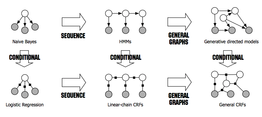
Hidden Markov models and beyond
Finally, hidden Markov models are to naive Bayes what conditional random fields are to softmax regression: the former in each pair builds upon the latter by modeling a sequence of labels. This graphic1 gives a bit more insight into these relationships:
Where does \(e\) come from?
Equation (2) states that the numerator of the softmax, i.e. the exponentiated linear combination of input elements, is equivalent to the unnormalized joint probability of our inputs and outputs as given by the Gibbs distribution factor product.
However, this only holds if one of the following two are true:
- Our factors are of the form \(e^{z}\).
- Our factors take any arbitrary form, and we "anticipate" that this form will be exponentiated within the softmax function.
Remember, the point of this exponentiation was to put our weighted input elements "on the arithmetic path to becoming valid probabilities," i.e. to make them strictly positive. This said, there is nothing (to my knowledge) that mandates that a factor produce a strictly positive number. So which came first — the chicken or the egg (the exponent or the softmax)?
In truth, I'm not actually sure, but I do believe we can safely treat the softmax numerator and an unnormalized Gibbs distribution as equivalent and simply settle on: call it what you will, we need an exponent in there somewhere to put this thing in \([0, 1]\).
Summary
This exercise has made the relationships between canonical machine learning models, activation functions and the basic axiom of conditional probability a whole lot clearer. For more information, please reference the resources below — especially Daphne Koller's material on probabilistic graphical models. Thanks so much for reading.
References: